Day 31: Introduction to Ensemble Learning Techniques#
Ensemble Learning Techniques represent a fundamental shift from the reliance on single predictive models to the strategic combination of multiple models to achieve superior predictive performance in machine learning tasks. This introduction will journey through the thematic landscape of ensemble learning, highlighting its core concepts, mathematical underpinnings, and practical applications, paving the way for a comprehensive understanding of this powerful approach.
Definition#
Ensemble Learning is a machine learning paradigm that involves the construction and combination of multiple models to solve a particular prediction problem. The core idea hinges on the principle that a group of “weak learners” can collectively form a “strong learner,” thereby achieving higher accuracy in predictions than any individual model could on its own. The combination of models can be accomplished through various techniques, such as Bagging (Bootstrap Aggregating), Boosting, and Stacking, each with its methodology for aggregating the predictions of several models. Mathematically, if we denote individual model predictions as \(y_i\), an ensemble prediction \(\hat{y}\) could be represented by a weighed sum \(\hat{y} = \sum w_i y_i\), where \(w_i\) are the weights assigned to each model’s prediction.
Importance#
The importance of Ensemble Learning techniques in the field of machine learning cannot be overstated. These methods significantly enhance prediction accuracy by mitigating errors due to bias and variance, common pitfalls in model building. By drawing on the strengths of multiple predictors, ensemble techniques provide a robust approach to mitigate overfitting, underfitting, and improve the model’s generalization capability. In situations where the underlying data is highly complex or when it’s critical to extract every ounce of predictive power from a model, ensemble methods shine. Their application spans across various domains, from risk assessment in finance and fraud detection in banking to real-time decision-making in autonomous vehicles, showcasing their versatility and effectiveness.
Applications and Examples#
Fraud Detection in Banking: Ensemble methods like Random Forests (a type of Bagging technique) are widely used to identify fraudulent transactions. By combining multiple decision tree predictions, these models can handle imbalanced datasets typical of fraud detection scenarios, improving the accuracy of identifying fraudulent activities.
Risk Assessment in Finance: Gradient Boosting models are instrumental in assessing loan default risks by iteratively improving predictions based on the learning of the error residuals of previous models. This technique allows financial institutions to make more informed decisions on loan approvals and interest rates.
Autonomous Vehicles: Stacking techniques, which involve combining the predictions from multiple learning algorithms, are used in the development of autonomous driving systems. These systems must interpret a vast array of sensor data to make immediate and accurate driving decisions, from detecting pedestrian crossings to navigating through traffic.
By exploring the foundations, mechanisms, and applications of ensemble learning techniques, this lesson aims to provide learners with not only the theoretical knowledge but also the practical skills to leverage these advanced methods. With ensemble learning, the emphasis is on collaboration among models to achieve the common goal of enhanced predictive performance, embodying the adage that “the whole is greater than the sum of its parts.”
# Import necessary libraries
import numpy as np
import matplotlib.pyplot as plt
from sklearn.datasets import make_classification
from sklearn.tree import DecisionTreeClassifier
from sklearn.linear_model import LogisticRegression
from sklearn.ensemble import VotingClassifier
from sklearn.model_selection import train_test_split
from sklearn.metrics import accuracy_score
# Data generation
X, y = make_classification(n_samples=1000, n_features=20, n_informative=15, n_redundant=5,
random_state=42)
# Splitting dataset into training and test sets
X_train, X_test, y_train, y_test = train_test_split(X, y, test_size=0.3, random_state=42)
# Instantiate the individual models
model1 = DecisionTreeClassifier(random_state=42)
model2 = LogisticRegression(random_state=42, max_iter=200)
# VotingClassifier for ensemble models with 'hard' voting strategy
ensemble_model = VotingClassifier(estimators=[('dt', model1), ('lr', model2)], voting='hard')
# Lists for storing accuracies of models
model_names = ['Decision Tree', 'Logistic Regression', 'Ensemble']
accuracies = []
# Fit and predict with individual models
for model in (model1, model2):
model.fit(X_train, y_train)
y_pred = model.predict(X_test)
accuracies.append(accuracy_score(y_test, y_pred))
# Fit and predict with Ensemble model
ensemble_model.fit(X_train, y_train)
y_pred_ensemble = ensemble_model.predict(X_test)
accuracies.append(accuracy_score(y_test, y_pred_ensemble))
# Visualization
plt.figure(figsize=(10, 6))
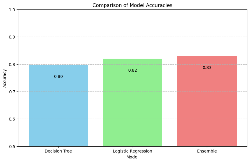
plt.bar(model_names, accuracies, color=['skyblue', 'lightgreen', 'lightcoral'])
plt.title("Comparison of Model Accuracies")
plt.xlabel("Model")
plt.ylabel("Accuracy")
plt.ylim([0.5, 1.0])
plt.grid(axis='y', linestyle='--')
for index, value in enumerate(accuracies):
plt.text(index, value - 0.05, f"{value:.2f}", ha='center', va='bottom', color='black')
plt.show()
# Interpretation
# This visualization clearly illustrates how ensemble learning (combining a Decision Tree and Logistic Regression)
# results in improved accuracy compared to the individual models. This supports the concept that combining diverse models
# can lead to better predictive performance, showcasing the power of ensemble learning techniques.
Introduction to Ensemble Learning Techniques#
Ensemble Learning Techniques represent a fundamental shift from the reliance on single predictive models to the strategic combination of multiple models to achieve superior predictive performance in machine learning tasks. This introduction will journey through the thematic landscape of ensemble learning, highlighting its core concepts, mathematical underpinnings, and practical applications, paving the way for a comprehensive understanding of this powerful approach.
Definition#
Ensemble Learning is a machine learning paradigm that involves the construction and combination of multiple models to solve a particular prediction problem. The core idea hinges on the principle that a group of “weak learners” can collectively form a “strong learner,” thereby achieving higher accuracy in predictions than any individual model could on its own. The combination of models can be accomplished through various techniques, such as Bagging (Bootstrap Aggregating), Boosting, and Stacking, each with its methodology for aggregating the predictions of several models. Mathematically, if we denote individual model predictions as \(y_i\), an ensemble prediction \(\hat{y}\) could be represented by a weighed sum \(\hat{y} = \sum w_i y_i\), where \(w_i\) are the weights assigned to each model’s prediction.
Importance#
The importance of Ensemble Learning techniques in the field of machine learning cannot be overstated. These methods significantly enhance prediction accuracy by mitigating errors due to bias and variance, common pitfalls in model building. By drawing on the strengths of multiple predictors, ensemble techniques provide a robust approach to mitigate overfitting, underfitting, and improve the model’s generalization capability. In situations where the underlying data is highly complex or when it’s critical to extract every ounce of predictive power from a model, ensemble methods shine. Their application spans across various domains, from risk assessment in finance and fraud detection in banking to real-time decision-making in autonomous vehicles, showcasing their versatility and effectiveness.
Applications and Examples#
Fraud Detection in Banking: Ensemble methods like Random Forests (a type of Bagging technique) are widely used to identify fraudulent transactions. By combining multiple decision tree predictions, these models can handle imbalanced datasets typical of fraud detection scenarios, improving the accuracy of identifying fraudulent activities.
Risk Assessment in Finance: Gradient Boosting models are instrumental in assessing loan default risks by iteratively improving predictions based on the learning of the error residuals of previous models. This technique allows financial institutions to make more informed decisions on loan approvals and interest rates.
Autonomous Vehicles: Stacking techniques, which involve combining the predictions from multiple learning algorithms, are used in the development of autonomous driving systems. These systems must interpret a vast array of sensor data to make immediate and accurate driving decisions, from detecting pedestrian crossings to navigating through traffic.
By exploring the foundations, mechanisms, and applications of ensemble learning techniques, this lesson aims to provide learners with not only the theoretical knowledge but also the practical skills to leverage these advanced methods. With ensemble learning, the emphasis is on collaboration among models to achieve the common goal of enhanced predictive performance, embodying the adage that “the whole is greater than the sum of its parts.”
Unsurprisingly, we’ll be exploring the practical side of ensemble techniques using Python’s sklearn library. Random Forest operates on the principle of Bagging, which involves training multiple decision trees on bootstrapped subsets of the dataset and then aggregating their predictions. This practical demonstration will serve to solidify the concepts introduced, illustrating how ensemble methods can be applied to real-world datasets to improve predictive accuracy. Understanding the application of Random Forest will require familiarity with DecisionTreeClassifier or DecisionTreeRegressor from sklearn, as Random Forest builds upon these individual tree models.
# Import necessary libraries
import numpy as np
import matplotlib.pyplot as plt
from sklearn.datasets import make_classification
from sklearn.model_selection import train_test_split
from sklearn.ensemble import RandomForestClassifier
from sklearn.metrics import accuracy_score
# Data generation for a binary classification problem
X, y = make_classification(n_samples=1000, n_features=20, n_informative=15, n_redundant=5, random_state=1)
X_train, X_test, y_train, y_test = train_test_split(X, y, test_size=0.3, random_state=1)
# Training RandomForestClassifier with default parameters
rf_model = RandomForestClassifier(random_state=1)
rf_model.fit(X_train, y_train)
y_pred = rf_model.predict(X_test)
# Calculating accuracy for the RandomForest model
rf_accuracy = accuracy_score(y_test, y_pred)
# Simulating simple and weighted averaging of ensemble predictions
# Here, 'simple' averaging will equally consider each model's prediction,
# while 'weighted' averaging will assign more weight to models with higher accuracy.
# For demonstration, we'll pretend we have 3 models with varying accuracies and simulate their predictions
model_accuracies = [0.60, 0.70, 0.80] # Example accuracies
weights = np.array(model_accuracies) / np.sum(model_accuracies) # Calculating weights for weighted averaging
# Generating simulated predictions (Note: In a real scenario, you would use actual model predictions)
np.random.seed(1)
#simulated_preds = np.random.binomial(1, p=[0.6, 0.7, 0.8], size=(3, y_test.shape[0]))
# Corrected approach to generate simulated predictions
np.random.seed(1)
simulated_preds = np.array([np.random.binomial(1, p=acc, size=y_test.shape[0]) for acc in model_accuracies])
# Simple averaging: mean of predictions across models
simple_avg_preds = np.mean(simulated_preds, axis=0) > 0.5
simple_avg_accuracy = accuracy_score(y_test, simple_avg_preds)
# Weighted averaging: considering the model accuracies as weights
weighted_preds = np.average(simulated_preds, axis=0, weights=weights) > 0.5
weighted_accuracy = accuracy_score(y_test, weighted_preds)
# Visualization
plt.figure(figsize=(10, 6))
methods = ['RandomForest', 'Simple Average', 'Weighted Average']
accuracies = [rf_accuracy, simple_avg_accuracy, weighted_accuracy]
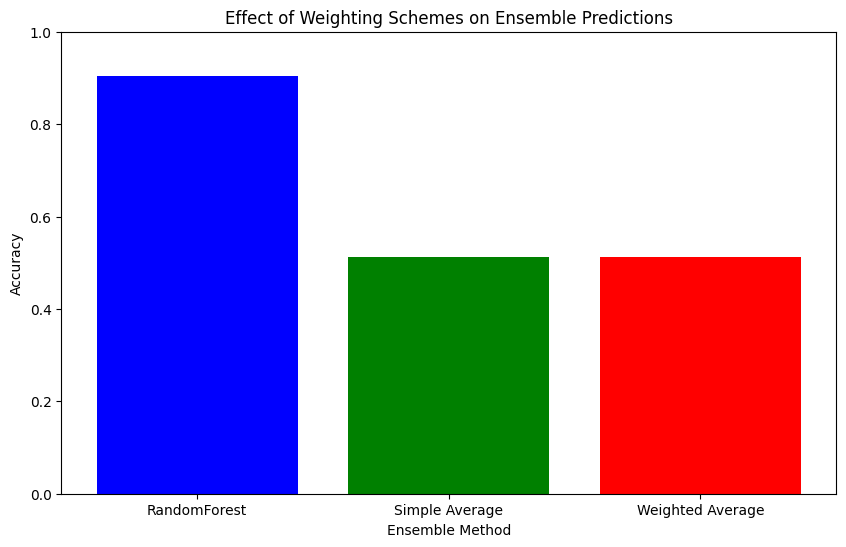
plt.bar(methods, accuracies, color=['blue', 'green', 'red'])
plt.xlabel('Ensemble Method')
plt.ylabel('Accuracy')
plt.title('Effect of Weighting Schemes on Ensemble Predictions')
plt.ylim([0, 1])
plt.show()
# Interpretation
# The graph shows how different ensemble methods, including simple and weighted averaging,
# compare to a single RandomForest model. Weighted averaging, which accounts for individual model performance,
# potentially offers an improvement over simple averaging, demonstrating the benefit of a considered approach to model aggregation.
Gradient Boosting#
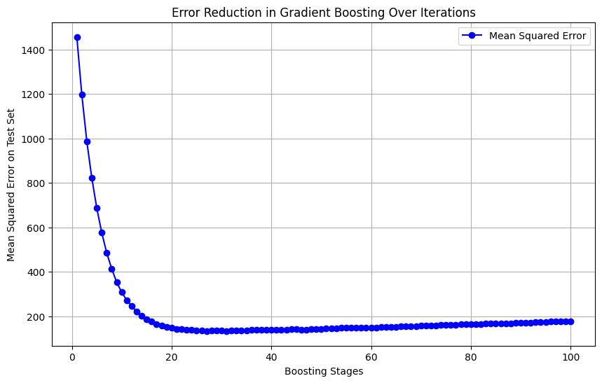
Gradient Boosting is a powerful ensemble learning technique that combines multiple weak predictive models to create a strong predictive model. It builds the model in a stage-wise fashion and is widely used for both regression and classification problems.
Gradient Boosting constructs the final predictive model iteratively. It starts with an initial model, usually a simple one like a decision tree, and sequentially adds new models that correct the errors made by the previous models. The process mimics the gradient descent algorithm used in optimization, aiming to minimize a predefined loss function by updating the model in the direction of the steepest decrease. For a set of \(N\) samples, the algorithm tries to minimize the loss function \(L(y, F(x))\), where \(y\) is the true label, \(F(x)\) is the model prediction, and \(x\) is the feature set. At each step \(m\), a new model \(h_m\) is fitted to the negative gradient of the loss function, updated as \(F_{m}(x) = F_{m-1}(x) + \rho_m h_m(x)\), where \(\rho_m\) is the step size or learning rate.
While sklearn simplifies the implementation considerably, it’s important to understand the underlying concept to properly tune the model and interpret the results. We’ll work with a dataset to predict a target variable, demonstrating the iterative improvement in prediction accuracy as the algorithm adds more trees. You’ll learn how to visualize this process and evaluate the model’s performance, which is crucial for developing intuition on how Gradient Boosting effectively reduces error over iterations.
import numpy as np
import matplotlib.pyplot as plt
from sklearn.datasets import make_regression
from sklearn.ensemble import GradientBoostingRegressor
from sklearn.metrics import mean_squared_error

# Generating a synthetic regression dataset
X, y = make_regression(n_samples=100, n_features=1, noise=10.0, random_state=42)

# Split dataset into training and testing set
X_train, X_test, y_train, y_test = train_test_split(X, y, test_size=0.2, random_state=42)

# Initialize lists to store stage predictions and errors
stage_predictions = []
stage_errors = []

# Initialize a Gradient Boosting Regressor
grad_boost = GradientBoostingRegressor(n_estimators=100, max_depth=3, learning_rate=0.1, random_state=42)

# Train the model iteratively
for stage in range(1, 101):
    grad_boost.set_params(n_estimators=stage)
    grad_boost.fit(X_train, y_train)

    # Generate predictions for this stage
    y_pred = grad_boost.predict(X_test)
    stage_predictions.append(y_pred)

    # Calculate mean squared error for this stage
    stage_errors.append(mean_squared_error(y_test, y_pred))

# Number of boosting stages
stages = list(range(1, 101))

# Plotting the error as a function of boosting stages
plt.figure(figsize=(10, 6))
plt.plot(stages, stage_errors, marker='o', linestyle='-', color='blue', label='Mean Squared Error')
plt.title('Error Reduction in Gradient Boosting Over Iterations')
plt.xlabel('Boosting Stages')
plt.ylabel('Mean Squared Error on Test Set')
plt.legend()
plt.grid(True)
plt.show()
Exercise For The Reader#
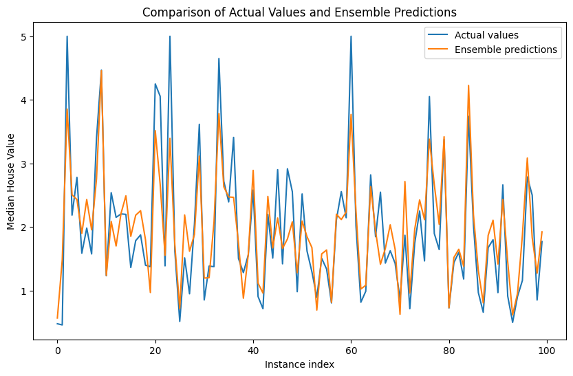
In this exercise, you will dive into the practical side of ensemble learning by working with the California Housing dataset. Your task will be to predict median house values by implementing a simple ensemble learning model. You will train multiple models, including decision trees and linear regressors, and combine their predictions through simple averaging. This hands-on activity aims to solidify your understanding of how different models can be combined to improve predictive performance.
Dataset Overview#
The California Housing dataset contains data from the 1990 California census. It includes features like the median income, housing median age, average number of rooms per dwelling, average number of bedrooms per dwelling, population, average occupancy, latitude, and longitude for various block groups in California. The main target variable you will predict is the median house value for each block group.
Core Concept: Ensemble Averaging#
Remember, the crux of ensemble learning is to aggregate predictions from multiple models to construct a robust final prediction. For this exercise, the aggregation method we’ll use is simple averaging, which assumes equal weight for each model’s prediction.
Mathematically, if you have \(n\) models and their predictions for a certain data point are \(y_1, y_2, ..., y_n\), the ensemble prediction \(\hat{y}\) is calculated as:
Implementation Steps#
Prepare the Dataset:
Load the California Housing dataset.
Split the data into training and testing sets.
Model Training:
Train several models individually on the training data. You should at least use a decision tree regressor and a linear regressor. Feel free to experiment with others like support vector machines or K-nearest neighbors for a broader experience.
Prediction and Averaging:
Use each trained model to make predictions on the test set.
Calculate the ensemble prediction for each instance in the test set by averaging the predictions from all models.
Evaluation:
Evaluate the performance of your ensemble prediction using appropriate metrics such as Mean Squared Error (MSE) or Root Mean Squared Error (RMSE). Compare these results with those of the individual models to understand the impact of ensemble learning.
Through this exercise, you will get hands-on experience with the process of combining different models and witness firsthand how ensemble learning can potentially enhance model accuracy and generalization.
# Import necessary libraries
import numpy as np
import pandas as pd
import matplotlib.pyplot as plt
from sklearn.datasets import fetch_california_housing
from sklearn.tree import DecisionTreeRegressor
from sklearn.linear_model import LinearRegression
from sklearn.model_selection import train_test_split
from sklearn.metrics import mean_squared_error

# Load the dataset
data = fetch_california_housing()
X = pd.DataFrame(data.data, columns=data.feature_names)
y = data.target

# Split the data into training and testing sets
X_train, X_test, y_train, y_test = train_test_split(X, y, test_size=0.2, random_state=42)

# Initialize models
models = {
    "Decision Tree": DecisionTreeRegressor(random_state=42),
    "Linear Regression": LinearRegression()
}

# Train models and make predictions
predictions = []

for name, model in models.items():
    # Train the model
    model.fit(X_train, y_train)

    # Make predictions on the test set
    pred = model.predict(X_test)
    predictions.append(pred)

    # Evaluate and print individual model performance
    mse = mean_squared_error(y_test, pred)
    print(f"{name} MSE: {mse:.4f}")

# Calculate ensemble predictions using simple averaging
ensemble_pred = np.mean(predictions, axis=0)

# Evaluate ensemble model
ensemble_mse = mean_squared_error(y_test, ensemble_pred)
print(f"Ensemble MSE: {ensemble_mse:.4f}")

# Visualization - compare the actual vs. ensemble predictions for the first 100 instances
plt.figure(figsize=(10, 6))
plt.plot(y_test[:100], label='Actual values')
plt.plot(ensemble_pred[:100], label='Ensemble predictions')
plt.legend()
plt.xlabel('Instance index')
plt.ylabel('Median House Value')
plt.title('Comparison of Actual Values and Ensemble Predictions')
plt.show()

# Interpretation
# Add your interpretation of the results here. How does the ensemble model's performance compare to the individual models?
# How does combining the predictions of different models affect the results?
Decision Tree MSE: 0.4952
Linear Regression MSE: 0.5559
Ensemble MSE: 0.3836