Day 9: Calculus - Integrals, Fundamental Theorems, and Applications in Machine Learning

Objective

Deepen your understanding of integrals in calculus, their foundational principles, and their profound applications, particularly in Machine Learning (ML). Learn how to perform basic integrations in Python and explore how integrals contribute to various ML techniques.

Prerequisites

• Proficiency in Python programming.

• Fundamental knowledge of algebra, pre-calculus concepts, and calculus.

• Eagerness to explore mathematical principles and apply them to real-world scenarios.

Introduction to Integrals

Integrals, pivotal in calculus, represent the accumulation of quantities, akin to summing up infinitesimally small pieces to find areas under curves or the total quantity accumulated over an interval. They play a crucial role not just in physics and engineering but also in data science and ML for understanding distributions, optimizing functions, and much more.

Mathematical Concept of Integrals

• Definite Integrals: Compute the accumulation of a quantity, such as the area under a curve from point a to point b. Mathematically, the definite integral of a function f(x) from a to b is denoted as:

\[∫^a_b f(x) dx\]

• Indefinite Integrals (Antiderivatives): Represent a family of functions whose derivatives give the original function. An indefinite integral of a function f(x) is represented as:

\[∫f(x) dx\]

Fundamental Theorems of Calculus

• First Fundamental Theorem: Connects differentiation and integration, asserting that if f is continuous on [a, b] and F is the indefinite integral of f on [a, b], then:

\[F(b)−F(a)=∫^a_bf(x) dxF(b)−F(a)=∫^a_b​f(x)dx\]

• Second Fundamental Theorem: Enables the evaluation of definite integrals by knowing an antiderivative of the function. If F is an antiderivative of continuous f on [a, b], then:

\[∫^a_b f(x) dx=F(b)−F(a)\]

Application of Integrals in Machine Learning

Integrals find extensive applications in ML and AI for:

• Optimization Problems: Integrals are used in calculating areas under the curve in ROC analysis, integral representations in loss functions, and in regularization terms to prevent overfitting.

• Understanding Data Distributions: Integrals help in defining continuous probability distributions, essential for calculating probabilities and expectations in statistical models.

• Deep Learning: In neural networks, integrals appear in backpropagation algorithms for computing gradients and in defining activation functions.

Implementing Integrals using Python

Python’s sympy library is excellent for symbolic mathematics, including integration.

# Step 1: Import Necessary Libraries

import sympy as sp
from sympy.abc import x 

# Step 2: Define the Function

# Choose a function to integrate. For instance, let's consider `f(x) = x^2`.
function = x**2

# Step 3: Compute the Indefinite Integral

indefinite_integral = sp.integrate(function, x)

print(f"The indefinite integral of f(x) = x^2 is: {indefinite_integral}")

The indefinite integral of f(x) = x^2 is: x**3/3

# Step 4: Compute the Definite Integral

# Calculate the definite integral of `f(x) = x^2` from `1` to `3`:
a, b = 1, 3
definite_integral = sp.integrate(function, (x, a, b))

print(f"The definite integral of f(x) = x^2 from {a} to {b} is: {definite_integral}")

The definite integral of f(x) = x^2 from 1 to 3 is: 26/3

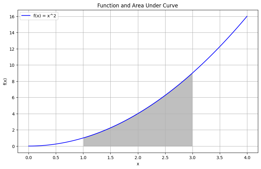
# Step 5: Visualizing the Function and its Integral

# Graph the function and the area under the curve between `x = 1` and `x = 3`:
import numpy as np
import matplotlib.pyplot as plt

# Define the function and integral as lambda functions
func_lambda = sp.lambdify(x, function, 'numpy')
integral_lambda = sp.lambdify(x, indefinite_integral, 'numpy')

# Generate x values
x_vals = np.linspace(0, 4, 100)
y_vals = func_lambda(x_vals)

# Plotting
plt.figure(figsize=(10, 6))
plt.plot(x_vals, y_vals, label='f(x) = x^2', color='blue')
plt.fill_between(x_vals, y_vals, where=[(x_val >= a and x_val <= b) for x_val in x_vals], color='gray', alpha=0.5)
plt.title('Function and Area Under Curve')
plt.xlabel('x')
plt.ylabel('f(x)')
plt.legend()
plt.grid(True)
plt.show()