
Day 6: Linear Algebra - Vector Operations in Python#
Introduction to Vectors#
What is a Vector?#
Definition: A vector is an ordered collection of values, often represented as an array or a list. In mathematics and programming, vectors are used to represent quantities that have both magnitude and direction. They are essential for various tasks in linear algebra, machine learning, and data analysis. A vector may be represented as:
\[\begin{split} \mathbf{v} = \begin{bmatrix} v_1 \\ v_2 \\ \vdots \\ v_n \end{bmatrix} \end{split}\]where \(n\) represents the number of components or elements in the vector.
Vectors in mathematics and physics possess both magnitude and direction:
Magnitude:
Magnitude represents the size or length of a vector.
It is denoted as \(||v||\) or \(|v|\) for a vector \((v)\).
Magnitude is a non-negative scalar value.
Direction:
Direction indicates where the vector points in space.
It specifies the orientation of the vector relative to a reference frame.
Direction can be represented using angles, unit vectors, or specific directions in a coordinate system.
To fully describe a vector, both its magnitude and direction are essential. While vectors have BOTH magnitude and direction. (i.e. A car traveling 60kph, NE), a scalar represents ONLY magnitude (i.e. distance, speed, measurement)
Importance: Vectors are of paramount importance in various scientific and engineering disciplines due to their versatility in representing both magnitude and direction. Just like matrices, vectors find wide-ranging applications:
In physics: Vectors are fundamental for describing physical quantities such as force, velocity, acceleration, and displacement. They help analyze the motion and interactions of objects.
In engineering: Vectors are used to represent the direction of loads, forces, and other structural elements in civil engineering, mechanical engineering, and electrical engineering.
In computer science: Vectors are indispensable in data structures and algorithms, particularly in machine learning and artificial intelligence, where they are used to represent and process data, such as feature vectors for classification tasks.
Vectors are a fundamental concept in mathematics and science, providing a concise and powerful means to represent a wide range of real-world phenomena and mathematical relationships. Understanding vectors is essential for tackling complex problems across various fields.
Vector Representation in Python#
Activity 1: Representing Vectors in Python#
Objective: Learn to create vectors using NumPy arrays.
Why Python and NumPy?: Python, with NumPy, is efficient and straightforward for handling mathematical operations, including vector manipulations.
import numpy as np
# Creating a vector
x = np.array([1, 3, 5, 7])

print("Vector v:", x)
Vector v: [1 3 5 7]
Indexing - Python is 0-indexed. When you are calling things from a ‘list’, vector, etc. The first number is actually at the 0 place.
print("Vector x at index 0:", x[0])
print("Vector x at index 1:", x[1])
Vector x at index 0: 1
Vector x at index 1: 3
Basic Vector Operations#
Activity 2: Basic Vector Operations#
Objective: Understand and perform vector addition, subtraction, and scalar multiplication.
Why This Matters: These operations are foundational for complex computations and are widely used in fields like physics.
import numpy as np

# Creating two vectors to represent data points
x1 = np.array([3, 4])
y1 = np.array([1, 2])

# Display the vectors
print("Vector 1:", x1)
print("Vector 2:", y1)
Vector 1: [3 4]
Vector 2: [1 2]
Vector addition, subtraction#
Why This Matters : Feature Engineering
Machine learning models often benefit from well-designed features. Vector addition and subtraction are crucial for feature engineering. For example, in image processing, subtracting background color vectors from images can enhance object recognition, making it easier to identify handwritten digits in optical character recognition (OCR).
For any vectors, whether it is x, y, z (of the same size/shape)
The following properties are true:
Vector addition is commutative \(x+y = y+x\)
Vector addition is associative: \((x+y)+z = x+(y+z)\). Therefore \(x+y+z\) is true.
Adding a zero vector to a vector has no effect: \(x+0 = 0+x = x\).
Subtracting a vector from itself as long as the size and shape are the same yields a zero vector \((x-x=0)\)
# Adding the vectors
sum = x1 + y1
print("Sum:", sum)

#OR

x_add = np.add(x1, y1)
print("Added Vectors:", x_add)

# Subtracting the vectors
difference = x1 - y1
print("Difference:", difference)
Sum: [4 6]
Added Vectors: [4 6]
Difference: [2 2]
Scalar or Vector Multiplication (One Vector x One Scalar)#
Why This Matters: Learning Rate Adjustment
In machine learning, gradient-based optimization algorithms, like stochastic gradient descent (SGD), require a learning rate. Scalar multiplication plays a pivotal role in adjusting the learning rate. For instance, when training a neural network, scaling the learning rate dynamically based on the progress of training helps avoid overshooting or slow convergence, ensuring effective model training.
For any vectors \(x, y\) and scalars \(a, b\)
The following properties are true:
Scalar-vector multiplication is commutative: \(ax = x * a\)
Scalar-vector multiplication is associative: \((ab)x = a(bx)\)
Scalar-vector mulitplication is distributive: \(a(x+y) = ax+ay, (x+y)a = xa+ya, (a+b)x=ax+bx\)
# Scalar multiplication
scaled = x1 * 2
print("Scaled:", scaled)

#OR

scalar = 2
x_scalar_mult = x1 * scalar
print("Scalar Multiplication:", x_scalar_mult)
Scaled: [6 8]
Scalar Multiplication: [6 8]
Vector Magnitude and Direction#
Activity 3: Vector Magnitude and Direction#
Objective: Calculate the magnitude and direction of a vector.
Real-world Relevance: Crucial in navigation, robotics, and physics for understanding vector length and orientation.
# Calculating magnitude and direction
magnitude = np.linalg.norm(x1)
direction = np.arctan2(x1[1], x1[0])

print("Magnitude of x1:", magnitude)
print("Direction of x1:", direction, "radians")
Magnitude of x1: 5.0
Direction of x1: 0.9272952180016122 radians
Advanced Vector Operations: Dot Product (Scalar Product)#
Why This Matters: Text Classification
Dot products are fundamental for text classification in natural language processing (NLP). By calculating dot products between word vectors and predefined sentiment vectors, you can determine the sentiment of a text. This enables automated sentiment analysis for large volumes of text data.
The dot product (also known as scalar product) is a way to multiply vectors that results in a scalar (a single number, not a vector).
Definition#
Given two vectors \(( \mathbf{x} \)) and \(( \mathbf{y} \)) in \(( \mathbb{R}^n \)) (n-dimensional real number space), the dot product is defined as:
where \(( x_i \)) and \(( y_i \)) are components of vectors \(( \mathbf{x} \)) and \(( \mathbf{y} \)), respectively.
Geometric Interpretation#
The dot product can also be expressed as:
where:
\(( |\mathbf{x}\)| ) is the magnitude of vector \(( \mathbf{x} \))
\(( |\mathbf{y}\)| ) is the magnitude of vector \(( \mathbf{y} \))
\(( \theta \)) is the angle between \(( \mathbf{x} \)) and \(( \mathbf{y} \))
Properties#
Commutative: \(( \mathbf{x} \cdot \mathbf{y} = \mathbf{y} \cdot \mathbf{x} \))
Distributive over vector addition: \(( \mathbf{x} \cdot (\mathbf{y} + \mathbf{a}) = \mathbf{x} \cdot \mathbf{y} + \mathbf{x} \cdot \mathbf{a} \))
Bilinear:\(( a(\mathbf{x} \cdot \mathbf{y}) = (a\mathbf{x}) \cdot \mathbf{y} = \mathbf{x} \cdot (a\mathbf{y}) \)), where \(( a \)) is a scalar.
Applications#
Determining Orthogonality: Two vectors are orthogonal (perpendicular) if their dot product is zero.
Projection: Projecting one vector onto another.
Finding Angles: The angle between two vectors can be determined using the dot product formula.
Example#
Let’s calculate the dot product of two vectors in \(( \mathbb{R}^3 \)):
The dot product is:
# Dot and cross product
dot_product = np.dot(x1, y1)
x1_3D = np.append(x1, 0)
y1_3D = np.append(y1, 0)

print("Dot Product:", dot_product)
Dot Product: 11
Advanced Vector Operations: Cross Product (Vector Product)#
Objective: Learn the dot and cross product of vectors.
Why This Matters: 3D Graphics and Physics
Cross products are crucial in 3D graphics and physics, particularly for calculating normals to surfaces, which are essential for lighting and rendering. They are also used in physics for finding torques and rotational vectors, helping to understand the dynamics of rotating bodies.
The cross product (also known as vector product) is an operation on two vectors in three-dimensional space, resulting in a vector that is perpendicular to both of the original vectors.
Definition#
Given two vectors \(( \mathbf{x} \)) and \(( \mathbf{y} \)) in \(( \mathby{R}^3 \)) (three-dimensional real number space), the cross product is defined as:
where \(( \mathbf{i}, \mathbf{j}, \mathbf{k} \)) are the unit vectors along the x, y, and z axes, and \(( a_1, a_2, a_3 \)) and \(( b_1, b_2, b_3 \)) are the components of vectors \(( \mathbf{x} \)) and \(( \mathbf{y} \)), respectively.
Geometric Interpretation#
The magnitude of the cross product is given by:
\(|\mathbf{x}| \cdot \mathbf{y}|\) = \(|\mathbf{x}| |\mathbf{y}| \sin(\theta)\)
where:
\(( |\mathbf{a}| \)) and \(( |\mathbf{b}| \)) are the magnitudes of vectors \(( \mathbf{x} \)) and \(( \mathbf{y} \))
\(( \theta \)) is the angle between \(( \mathbf{x} \)) and \(( \mathbf{y} \))
The direction of \(( \mathbf{x} \cdot \mathbf{y} \)) is perpendicular to the plane formed by \(( \mathbf{x} \)) and \(( \mathbf{y} \)), determined by the right-hand rule.
Properties#
Non-Commutative: \(( \mathbf{x} \cdot \mathbf{y} = -(\mathbf{y} \cdot \mathbf{x}) \))
Distributive over vector addition: \(( \mathbf{x} \cdot (\mathbf{y} + \mathbf{c}) = \mathbf{x} \cdot \mathbf{y} + \mathbf{x} \cdot \mathbf{c} \))
Not associative: \(( \mathbf{x} \cdot (\mathbf{y} \cdot \mathbf{c}) \neq (\mathbf{x} \cdot \mathbf{y}) \cdot \mathbf{c} \))
Applications#
Normal Vector Calculation: Computing a vector perpendicular to a plane in 3D space.
Torque: In physics, the cross product is used to determine the torque exerted by a force.
Rotational Vectors: Understanding the rotation of objects in three-dimensional space.
Example#
Let’s calculate the cross product of two vectors in \(( \mathbb{R}^3 \)):
The cross product is:
Simplifying this, we get:
cross_product = np.cross(x1_3D, y1_3D)
print("Cross Product:", cross_product)
Cross Product: [0 0 2]
Vector Norm#
Mathematical Formula
L2 Norm: \((|\mathbf{v}\|_2 = \sqrt{v_1^2 + v_2^2 + \ldots + v_n^2})\)
Why This Matters:
Vector norms are used in machine learning for regularization and similarity calculations.
Practical Example in Python
To calculate the L2 norm of a vector in Python, you can use the numpy library:
vector_v = np.array([3, 4])
l2_norm = np.linalg.norm(vector_v)

print(l2_norm)
5.0
Real-world Application: Vector in Computer Graphics#
Coding Activity: Vector in Graphics#
Objective: Use vectors to simulate 2D graphical movement.
Why It’s Important: Understanding vector representation and manipulation in digital space is fundamental in computer graphics and game development.
Simulating 2D movement with vectors#
position = np.array([0, 0])
movement = np.array([1, 1])
new_position = position + movement

print("New Position:", new_position)
New Position: [1 1]
Physics and Engineering Applications of Vectors#
Understanding Forces and Movements:
Application in Physics: Vectors represent forces and movements.
Why It’s Important: Predicting object movements under various conditions is crucial in mechanical and aerospace engineering.
import numpy as np

# Representing a force vector
force = np.array([2, 5])  # Force vector with 2 units in the x-direction and 5 units in the y-direction
print("Force Vector:", force)
Force Vector: [2 5]
Structural Analysis:
Engineering Application: Vectors in civil engineering analyze forces on structures.
Significance: Ensures safety and stability of structures like bridges and buildings.
Machine Learning and Data Science#
Vectors in Data Representation:
Application: Vectors represent data points in algorithms, with the dot product measuring similarity, important in clustering and classification.
Why It Matters: Crucial for developing accurate models in machine learning.
Optimizing Performance:
Data Science Utilization: Efficient vector manipulation optimizes complex data analyses.
Importance: In big data, efficiency enables quicker and more precise data processing.
Advanced Topics in Vector Operations#
Eigenvalues and Eigenvectors:
Concept: Eigenvectors scale without changing direction under a linear transformation, while eigenvalues are the scalars of this scaling.
Application: Crucial in systems of linear equations and machine learning algorithms.
Summary and Concluding Thoughts#
Vectors are more than abstract mathematical concepts; they are practical tools across disciplines. Understanding vectors enables us to model and solve complex problems, from infrastructure design to advancements in machine learning and quantum computing. Their simplicity and versatility make them indispensable in STEM fields.
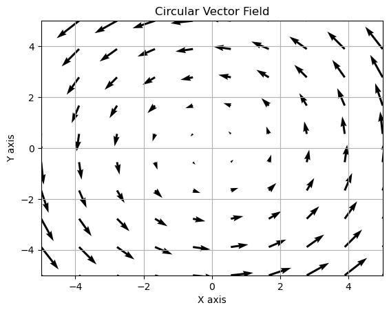
Activity: Vector Field Visualization for Beginners#
Objective: Create a simple 2D vector field visualization using Python. Duration: Approximately 20 minutes Tools Required: Python, basic Python syntax knowledge.
Step 1: Import necessary libraries#
import numpy as np
import matplotlib.pyplot as plt
Step 2: Create a grid#
x = np.linspace(-5, 5, 10)
y = np.linspace(-5, 5, 10)
X, Y = np.meshgrid(x, y)
Step 3: Define the vector field#
U and V are the components of the vector
U = -Y  # Negative Y component for circular pattern
V = X   # X component for circular pattern
Step 4: Plot the vector field#
plt.quiver(X, Y, U, V)
Step 5: Formatting the plot#
plt.xlim(-5, 5)
plt.ylim(-5, 5)
plt.title("Circular Vector Field")
plt.xlabel("X axis")
plt.ylabel("Y axis")
plt.grid()
Step 6: Display the plot#
plt.show()
# Step 1: Import necessary libraries
import numpy as np
import matplotlib.pyplot as plt

# Step 2: Create a grid
x = np.linspace(-5, 5, 10)
y = np.linspace(-5, 5, 10)
X, Y = np.meshgrid(x, y)

# Step 3: Define the vector field
# U and V are the components of the vector
U = -Y  # Negative Y component for circular pattern
V = X   # X component for circular pattern

# Step 4: Plot the vector field
plt.quiver(X, Y, U, V)

# Step 5: Formatting the plot
plt.xlim(-5, 5)
plt.ylim(-5, 5)
plt.title("Circular Vector Field")
plt.xlabel("X axis")
plt.ylabel("Y axis")
plt.grid()

# Step 6: Display the plot
plt.show()
Hands-On Project: Implementing and Visualizing Vector Operations#
Project Objective:
To apply the concept of vector operations in a practical scenario and visualize the results using Python.
Project Steps:
Create Multiple Vectors:
Represent different data points as vectors.
Perform addition, subtraction, and scalar multiplication.
Calculate and Visualize the Dot Product:
Calculate the dot product of vectors to understand their similarity.
Plot these vectors to visualize how the dot product represents the angle between them.
Project Code - Solution
# Hands-On Project: Vector Operations and Visualization
import numpy as np
import matplotlib.pyplot as plt
# Step 1: Create vectors
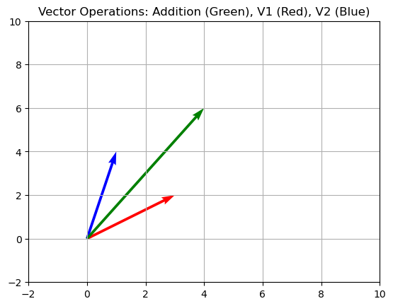
v1 = np.array([3, 2])
v2 = np.array([1, 4])
# Perform operations
v_add = np.add(v1, v2)
v_sub = np.subtract(v1, v2)
scalar = 3
v_scalar_mult = v1 * scalar
# Step 2: Dot product
dot_product = np.dot(v1, v2)
# Visualization
plt.quiver(0, 0, v1[0], v1[1], angles='xy', scale_units='xy', scale=1, color='r')
plt.quiver(0, 0, v2[0], v2[1], angles='xy', scale_units='xy', scale=1, color='b')
plt.quiver(0, 0, v_add[0], v_add[1], angles='xy', scale_units='xy', scale=1, color='g')
plt.xlim(-2, 10)
plt.ylim(-2, 10)
plt.grid()
plt.title('Vector Operations: Addition (Green), V1 (Red), V2 (Blue)')
plt.show()
# Print results
print("Added Vectors:", v_add)
print("Subtracted Vectors:", v_sub)
print("Scalar Multiplication:", v_scalar_mult)
print("Dot Product:", dot_product)
# Hands-On Project: Vector Operations and Visualization

import numpy as np
import matplotlib.pyplot as plt

# Step 1: Create vectors
v1 = np.array([3, 2])
v2 = np.array([1, 4])

# Perform operations
v_add = np.add(v1, v2)
v_sub = np.subtract(v1, v2)
scalar = 3
v_scalar_mult = v1 * scalar

# Step 2: Dot product
dot_product = np.dot(v1, v2)

# Visualization
plt.quiver(0, 0, v1[0], v1[1], angles='xy', scale_units='xy', scale=1, color='r')
plt.quiver(0, 0, v2[0], v2[1], angles='xy', scale_units='xy', scale=1, color='b')
plt.quiver(0, 0, v_add[0], v_add[1], angles='xy', scale_units='xy', scale=1, color='g')
plt.xlim(-2, 10)
plt.ylim(-2, 10)
plt.grid()
plt.title('Vector Operations: Addition (Green), V1 (Red), V2 (Blue)')
plt.show()

# Print results
print("Added Vectors:", v_add)
print("Subtracted Vectors:", v_sub)
print("Scalar Multiplication:", v_scalar_mult)
print("Dot Product:", dot_product)
Added Vectors: [4 6]
Subtracted Vectors: [ 2 -2]
Scalar Multiplication: [9 6]
Dot Product: 11
Further Resources#
Khan Academy’s Linear Algebra Course: Vectors and spaces
NumPy Documentation: NumPy for Vector Operations
Matplotlib Documentation: Matplotlib for Plotting