
Day 14: Data Normalization and Scaling using Python#
Objective#
Explore data normalization and feature scaling in Python, emphasizing the complete mathematical principles underlying these techniques, and understand their practical implications in data preprocessing for machine learning models.
Prerequisites#
Intermediate Python, Pandas, NumPy, and Scikit-Learn skills.
Basic understanding of statistical concepts and linear algebra.
Dataset: 100daysofml/100daysofml.github.io
Introduction to Data Normalization and Scaling#
Data normalization and scaling are essential preprocessing techniques in data analysis and machine learning. They ensure consistent data representation across features, improving the performance and interpretability of machine learning algorithms. By modifying feature scales, these techniques help in stabilizing model training and enhancing algorithm convergence speed.
Understanding Scaling Types#
Z-Score Normalization (Standardization)
Min-Max Scaling
Comprehensive Mathematical Foundations#
Z-Score Normalization (Standardization)#
Concept: Transforms data to have zero mean \((μ = 0)\) and unit variance \((σ² = 1)\).
Formula: \(Z=(X−μ)σZ=σ(X−μ)\)
Where XX is the original value, μμ is the mean, and σσ is the standard deviation.
Mathematical Rationale:
By subtracting the mean, the data is centered around zero.
Dividing by the standard deviation scales the data so that the variance is normalized.
Ideal for features following a Gaussian distribution or when the algorithm assumes Gaussian distribution (e.g., Linear Regression, Logistic Regression, Linear Discriminant Analysis).
Pros:
Less affected by outliers.
Keeps useful information about outliers.
Cons:
Not bound to a specific range.
Use Case: Algorithms that assume data is Gaussian (e.g., Linear Regression, Gaussian Naive Bayes).
Min-Max Scaling#
Concept: Rescales the range of features to [0, 1].
Formula: \(Xnorm=(X−Xmin)(Xmax−Xmin)Xnorm\)=(Xmax\(−Xmin\))(X−Xmin\()\)
Where XX is the original value, \(XminXmin\) and \(XmaxXmax\) are the minimum and maximum values.
Mathematical Rationale:
Ensures that all features contribute equally to the result.
Useful when algorithms are sensitive to the scale of input data (e.g., K-Nearest Neighbors, Neural Networks).
Prevents features with larger ranges from overpowering those with smaller ranges.
Pros:
Bound to a specific range.
Preserves relationships in data.
Cons:
Sensitive to outliers.
Use Case: Algorithms sensitive to input scale (e.g., Neural Networks, KNN).
Hands-On Activities with the Iris Dataset#
Implementing Z-Score Normalization#
Implement Z-Score Normalization and Min-Max Scaling using the StandardScaler and MinMaxScaler from Scikit-Learn, respectively. Tasks include examining the distribution of features before and after scaling, and comparing how scaling alters the range of values in features.
from sklearn.datasets import load_iris
from sklearn.preprocessing import StandardScaler
import pandas as pd

iris = load_iris()
iris_data = pd.DataFrame(iris.data, columns=iris.feature_names)
scaler = StandardScaler()
iris_standardized = scaler.fit_transform(iris_data)
Task: Examine the distribution of any feature before and after standardization.
Implementing Min-Max Scaling#
from sklearn.preprocessing import MinMaxScaler

min_max_scaler = MinMaxScaler()
iris_min_max_scaled = min_max_scaler.fit_transform(iris_data)
Task: Compare how min-max scaling alters the range of values in a feature.
Visualization and Analysis Post Data Normalization and Scaling#
Objective#
To visually and analytically assess the impact of normalization and scaling on the data’s distribution and inter-feature relationships.
Importance of Visualization#
Understanding Data Transformation: Visualization helps in comprehending how normalization and scaling alter the data.
Model Readiness Check: It ensures that the data is appropriately scaled or normalized for specific machine learning models.
Implementing Z-Score Normalization#
Load the dataset:
import pandas as pd
iris_data = pd.read_csv('Iris.csv')
print(iris_data.head())
Implement Z-Score Normalization:
from sklearn.preprocessing import StandardScaler
scaler = StandardScaler()
iris_standardized = scaler.fit_transform(iris_data.iloc[:, :-1])  # Assuming last column is target
Tasks:
Examine distribution of features before and after standardization.
Implement Min-Max Scaling:
from sklearn.preprocessing import MinMaxScalermin_max_scaler = MinMaxScaler()
iris_min_max_scaled = min_max_scaler.fit_transform(iris_data.iloc[:, :-1])
Tasks:
Compare how min-max scaling alters the range of values in features.
Visualization and Analysis Post Data Normalization and Scaling#
Visualization Techniques#
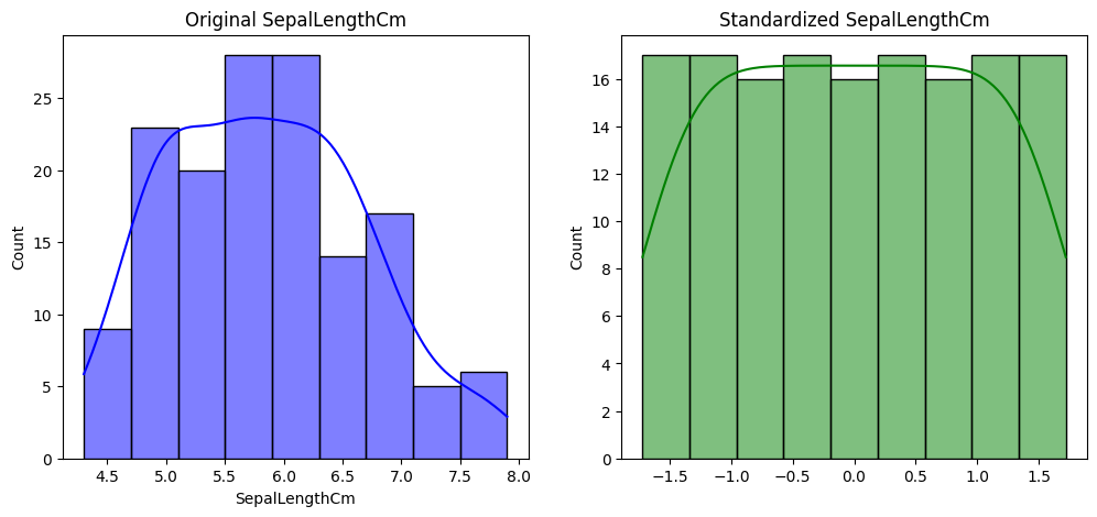
Histograms and Density Plots:
Show distribution of features before and after normalization or scaling.
Example:
import seaborn as sns
import matplotlib.pyplot as plt

feature = 'SepalLengthCm'
plt.figure(figsize=(12, 5))
plt.subplot(1, 2, 1)
sns.histplot(iris_data[feature], kde=True, color='blue')
plt.title(f'Original {feature}')

plt.subplot(1, 2, 2)
sns.histplot(iris_standardized[:, 0], kde=True, color='green')  # Adjust index accordingly
plt.title(f'Standardized {feature}')
plt.show()
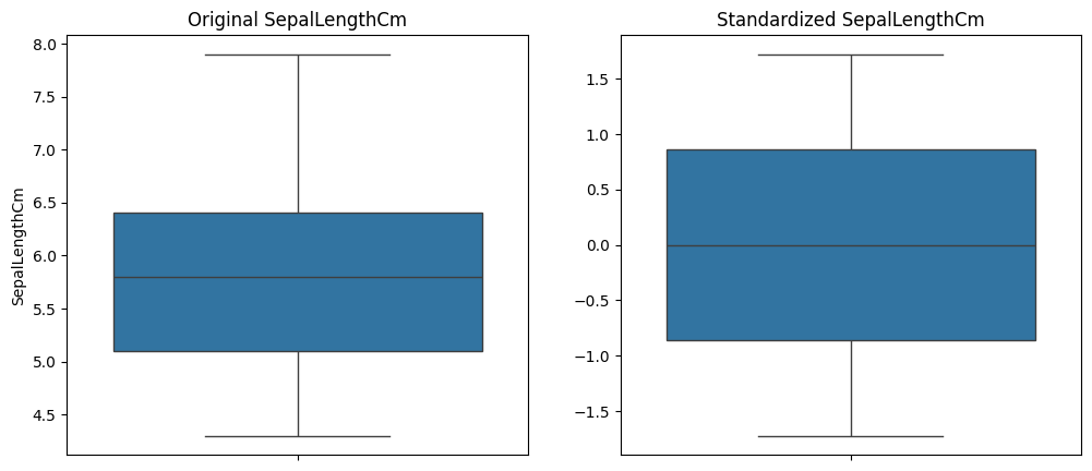
Box Plots:
Show spread and central tendency of the data.
Example:
plt.figure(figsize=(12, 5))
plt.subplot(1, 2, 1)
sns.boxplot(data=iris_data, y=feature)
plt.title(f'Original {feature}')

plt.subplot(1, 2, 2)
sns.boxplot(y=iris_standardized[:, 0])  # Adjust index accordingly
plt.title(f'Standardized {feature}')
plt.show()
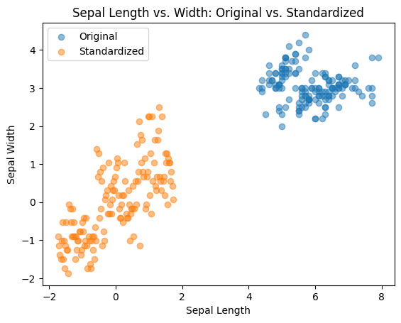
Scatter Plots:
Observe relationship between two features.
Example:
plt.scatter(iris_data['SepalLengthCm'], iris_data['SepalWidthCm'], alpha=0.5, label='Original')
plt.scatter(iris_standardized[:, 0], iris_standardized[:, 1], alpha=0.5, label='Standardized')  # Adjust indices accordingly
plt.xlabel('Sepal Length')
plt.ylabel('Sepal Width')
plt.title('Sepal Length vs. Width: Original vs. Standardized')
plt.legend()
plt.show()
Analytical Assessment Post-Scaling#
Statistical Summary:
Compare key statistics (mean, standard deviation, range) before and after scaling.
Use
describe()function in Pandas.
Correlation Analysis:
Assess changes in inter-feature correlations post-scaling.
Use
corr()function in Pandas.
Model Performance Evaluation:
Compare accuracy, precision, and recall before and after scaling.
Train models on original, standardized, and min-max scaled data.
Best Practices and Considerations#
Data Leakage: Fit scalers on the training set only to prevent information leakage.
Train/Test Splitting: Split data before preprocessing to avoid data snooping.
Choosing the Right Method: Consider data distribution, algorithm requirements, and presence of outliers when choosing a scaling method.
import pandas as pd
iris_data = pd.read_csv('Iris.csv')
print(iris_data.head())
   Id  SepalLengthCm  SepalWidthCm  PetalLengthCm  PetalWidthCm      Species
0   1            5.1           3.5            1.4           0.2  Iris-setosa
1   2            4.9           3.0            1.4           0.2  Iris-setosa
2   3            4.7           3.2            1.3           0.2  Iris-setosa
3   4            4.6           3.1            1.5           0.2  Iris-setosa
4   5            5.0           3.6            1.4           0.2  Iris-setosa
from sklearn.preprocessing import StandardScaler
scaler = StandardScaler()
iris_standardized = scaler.fit_transform(iris_data.iloc[:, :-1])  # Assuming last column is target
from sklearn.preprocessing import MinMaxScaler
min_max_scaler = MinMaxScaler()
iris_min_max_scaled = min_max_scaler.fit_transform(iris_data.iloc[:, :-1])
import seaborn as sns
import matplotlib.pyplot as plt

feature = 'SepalLengthCm'
plt.figure(figsize=(12, 5))
plt.subplot(1, 2, 1)
sns.histplot(iris_data[feature], kde=True, color='blue')
plt.title(f'Original {feature}')

plt.subplot(1, 2, 2)
sns.histplot(iris_standardized[:, 0], kde=True, color='green')  # Adjust index accordingly
plt.title(f'Standardized {feature}')
plt.show()
plt.figure(figsize=(12, 5))
plt.subplot(1, 2, 1)
sns.boxplot(data=iris_data, y=feature)
plt.title(f'Original {feature}')

plt.subplot(1, 2, 2)
sns.boxplot(y=iris_standardized[:, 0])  # Adjust index accordingly
plt.title(f'Standardized {feature}')
plt.show()
plt.scatter(iris_data['SepalLengthCm'], iris_data['SepalWidthCm'], alpha=0.5, label='Original')
plt.scatter(iris_standardized[:, 0], iris_standardized[:, 1], alpha=0.5, label='Standardized')  # Adjust indices accordingly
plt.xlabel('Sepal Length')
plt.ylabel('Sepal Width')
plt.title('Sepal Length vs. Width: Original vs. Standardized')
plt.legend()
plt.show()
Additional Resources (Train/Test Splitting | Data Leakage)#
https://machinelearningmastery.com/data-preparation-without-data-leakage/
https://www.analyticsvidhya.com/blog/2023/11/train-test-validation-split/
https://machinelearningmastery.com/train-test-split-for-evaluating-machine-learning-algorithms/
Day 14: Activity#
Step 1: Import necessary libraries#
Step 2: Load and Explore the Dataset#
Dataset: 100daysofml/100daysofml_notebooks
Step 3: Preprocess the Data#
Step 4: Split the Data into Training and Testing Sets#
Step 5: Apply Z-Score Normalization (Standardization)#
Step 6: Apply Min-Max Scaling#
Step 7: Visualize and Analyze the Effect of Scaling#
Step 8: Statistical Summary Comparison#
#Step 1: Import Necessary Libraries

import pandas as pd
import numpy as np
from sklearn.model_selection import train_test_split
from sklearn.preprocessing import StandardScaler, MinMaxScaler
import matplotlib.pyplot as plt
import seaborn as sns
#Step 2: Load and Explore the Dataset

# Load the dataset
titanic_data = pd.read_csv('titanic.csv')

# Display the first few rows of the dataset

print(titanic_data.head())

# Display summary statistics

print("\nSummary Statistics:")
print(titanic_data.describe())


# Check for missing values
print("\nMissing Values:")
print(titanic_data.isnull().sum())
   PassengerId  Pclass                                          Name     Sex  \
0          892       3                              Kelly, Mr. James    male
1          893       3              Wilkes, Mrs. James (Ellen Needs)  female
2          894       2                     Myles, Mr. Thomas Francis    male
3          895       3                              Wirz, Mr. Albert    male
4          896       3  Hirvonen, Mrs. Alexander (Helga E Lindqvist)  female

    Age  SibSp  Parch   Ticket     Fare Cabin Embarked  Survived
0  34.5      0      0   330911   7.8292   NaN        Q         0
1  47.0      1      0   363272   7.0000   NaN        S         1
2  62.0      0      0   240276   9.6875   NaN        Q         0
3  27.0      0      0   315154   8.6625   NaN        S         0
4  22.0      1      1  3101298  12.2875   NaN        S         1

Summary Statistics:
       PassengerId      Pclass         Age       SibSp       Parch  \
count   418.000000  418.000000  332.000000  418.000000  418.000000
mean   1100.500000    2.265550   30.272590    0.447368    0.392344
std     120.810458    0.841838   14.181209    0.896760    0.981429
min     892.000000    1.000000    0.170000    0.000000    0.000000
25%     996.250000    1.000000   21.000000    0.000000    0.000000
50%    1100.500000    3.000000   27.000000    0.000000    0.000000
75%    1204.750000    3.000000   39.000000    1.000000    0.000000
max    1309.000000    3.000000   76.000000    8.000000    9.000000

             Fare    Survived
count  417.000000  418.000000
mean    35.627188    0.385167
std     55.907576    0.487218
min      0.000000    0.000000
25%      7.895800    0.000000
50%     14.454200    0.000000
75%     31.500000    1.000000
max    512.329200    1.000000

Missing Values:
PassengerId      0
Pclass           0
Name             0
Sex              0
Age             86
SibSp            0
Parch            0
Ticket           0
Fare             1
Cabin          327
Embarked         0
Survived         0
dtype: int64
#Step 3: Preprocess the Data

# Handle missing values, encode categorical variables if necessary, and select features for scaling.

# Handling missing values (simple example by filling with median or mode)titanic_data['Age'].fillna(titanic_data['Age'].median(), inplace=True)
titanic_data['Embarked'].fillna(titanic_data['Embarked'].mode()[0], inplace=True)

# Select features for scaling (numeric features)
features = ['Pclass', 'Age', 'SibSp', 'Parch', 'Fare']
X = titanic_data[features]

# If 'Survived' is the target variable
y = titanic_data['Survived']
/tmp/ipykernel_1401614/1279951594.py:6: FutureWarning: A value is trying to be set on a copy of a DataFrame or Series through chained assignment using an inplace method.
The behavior will change in pandas 3.0. This inplace method will never work because the intermediate object on which we are setting values always behaves as a copy.

For example, when doing 'df[col].method(value, inplace=True)', try using 'df.method({col: value}, inplace=True)' or df[col] = df[col].method(value) instead, to perform the operation inplace on the original object.


  titanic_data['Embarked'].fillna(titanic_data['Embarked'].mode()[0], inplace=True)
#Step 4: Split the Data into Training and Testing Sets

X_train, X_test, y_train, y_test = train_test_split(X, y, test_size=0.2, random_state=42)
#Step 5: Apply Z-Score Normalization (Standardization)

scaler = StandardScaler()
X_train_standardized = scaler.fit_transform(X_train)
X_test_standardized = scaler.transform(X_test)
#Step 6: Apply Min-Max Scaling

min_max_scaler = MinMaxScaler()
X_train_min_max = min_max_scaler.fit_transform(X_train)
X_test_min_max = min_max_scaler.transform(X_test)
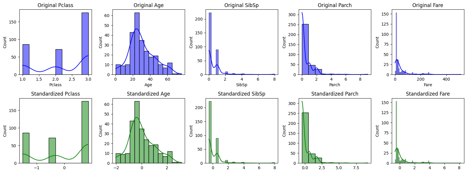
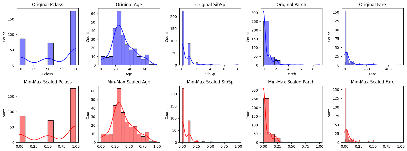
#Step 7: Visualize and Analyze the Effect of Scaling

#Visualize the effect of Z-Score Normalization and Min-Max Scaling on the feature distributions.

#Visualize the distribution of features before and after Z-Score Normalization
plt.figure(figsize=(16, 6))
for i, feature in enumerate(features):
    plt.subplot(2, len(features), i+1)
    sns.histplot(X_train[feature], kde=True, color='blue', label='Original')
    plt.title(f'Original {feature}')
    plt.subplot(2, len(features), len(features)+i+1)
    sns.histplot(X_train_standardized[:, i], kde=True, color='green', label='Standardized')
    plt.title(f'Standardized {feature}')
plt.tight_layout()
plt.show()

# Visualize the distribution of features before and after Min-Max Scaling
plt.figure(figsize=(16, 6))
for i, feature in enumerate(features):
    plt.subplot(2, len(features), i+1)
    sns.histplot(X_train[feature], kde=True, color='blue', label='Original')
    plt.title(f'Original {feature}')
    plt.subplot(2, len(features), len(features)+i+1)
    sns.histplot(X_train_min_max[:, i], kde=True, color='red', label='Min-Max Scaled')
    plt.title(f'Min-Max Scaled {feature}')
plt.tight_layout()
plt.show()
#Step 8: Statistical Summary Comparison

#Compare the statistical summary before and after scaling.

# Statistical summary before scalingprint("Statistical Summary before scaling:")
print(X_train.describe())

# Statistical summary after Z-Score Normalization
print("\nStatistical Summary after Z-Score Normalization:")
print(pd.DataFrame(X_train_standardized, columns=features).describe())

# Statistical summary after Min-Max Scaling
print("\nStatistical Summary after Min-Max Scaling:")
print(pd.DataFrame(X_train_min_max, columns=features).describe())
           Pclass         Age       SibSp       Parch        Fare
count  334.000000  262.000000  334.000000  334.000000  333.000000
mean     2.269461   30.115763    0.470060    0.404192   36.909135
std      0.844961   14.655775    0.944719    0.937113   58.054690
min      1.000000    0.330000    0.000000    0.000000    0.000000
25%      1.000000   21.000000    0.000000    0.000000    7.887500
50%      3.000000   27.000000    0.000000    0.000000   14.454200
75%      3.000000   39.000000    1.000000    0.000000   32.500000
max      3.000000   76.000000    8.000000    9.000000  512.329200

Statistical Summary after Z-Score Normalization:
             Pclass           Age         SibSp         Parch          Fare
count  3.340000e+02  2.620000e+02  3.340000e+02  3.340000e+02  3.330000e+02
mean   2.233742e-16  2.711995e-17  2.127373e-17 -3.722904e-17 -4.267524e-17
std    1.001500e+00  1.001914e+00  1.001500e+00  1.001500e+00  1.001505e+00
min   -1.504644e+00 -2.036246e+00 -4.983123e-01 -4.319630e-01 -6.367217e-01
25%   -1.504644e+00 -6.231816e-01 -4.983123e-01 -4.319630e-01 -5.006539e-01
50%    8.658800e-01 -2.130032e-01 -4.983123e-01 -4.319630e-01 -3.873714e-01
75%    8.658800e-01  6.073537e-01  5.617915e-01 -4.319630e-01 -7.606225e-02
max    8.658800e-01  3.136788e+00  7.982518e+00  9.186412e+00  8.201500e+00

Statistical Summary after Min-Max Scaling:
           Pclass         Age       SibSp       Parch        Fare
count  334.000000  262.000000  334.000000  334.000000  333.000000
mean     0.634731    0.393627    0.058757    0.044910    0.072042
std      0.422481    0.193680    0.118090    0.104124    0.113315
min      0.000000    0.000000    0.000000    0.000000    0.000000
25%      0.000000    0.273160    0.000000    0.000000    0.015395
50%      1.000000    0.352451    0.000000    0.000000    0.028213
75%      1.000000    0.511035    0.125000    0.000000    0.063436
max      1.000000    1.000000    1.000000    1.000000    1.000000
Additional Resources (Data Normalization & Scaling)#
https://www.kaggle.com/code/alexisbcook/scaling-and-normalization
https://www.simplilearn.com/normalization-vs-standardization-article