
Day 8: Calculus - Derivatives, Concept and Applications#
Objective#
Enhance your understanding of derivatives in calculus, their mathematical essence, real-world significance, and practical applications in machine learning and AI. Learn how to implement and visualize derivatives using Python, and grasp their role in various ML/AI algorithms.
Prerequisites#
Basic Python programming skills.
Knowledge of algebra and pre-calculus concepts.
Curiosity and willingness to explore mathematical ideas.
Introduction to Derivatives#
In calculus, a derivative represents how a function changes as its input changes. It’s akin to understanding not just your position while driving a car, but how your speed varies over time. In machine learning and AI, this concept of ‘rate of change’ is pivotal in optimizing models, making predictions, and understanding the relationship between variables.
Mathematical Concept of Derivatives#
Mathematically, the derivative of a function \(f(x)\) at a point \(x = a\) is defined as:
This limit, if it exists, provides the instantaneous rate of change of the function at \(x = a\), effectively giving the slope of the tangent line to the curve at that point.
What are Derivatives?#
Derivatives are a fundamental concept in calculus that allow us to understand how a function changes as its input (independent variable) changes. They provide information about the rate of change, slope, and behavior of functions. In this lesson, we’ll explore the concept of derivatives, their importance, and how they are used in various fields, including machine learning.
Understanding Rates of Change#
Imagine you are driving a car, and you want to know how fast your speed is changing at a specific moment. This rate of change in speed is precisely what derivatives help us calculate. Whether it’s measuring the speed of a car, the growth of a population, or the behavior of a stock price, derivatives are essential for understanding these changes.
Calculating Derivatives#
The Slope of a Tangent Line#
One way to think about derivatives is in terms of slopes. Given a curve representing a function, the derivative at a particular point on the curve provides the slope of the tangent line to the curve at that point. This tangent line represents the instantaneous rate of change at that specific moment.
Derivative Notation#
In mathematical notation, the derivative of a function is often denoted as \((f'(x)\)) or \((\frac{df}{dx}\)). Here’s what this notation means:
\((f'(x)\)): Represents the derivative of the function \((f\)) with respect to the variable \((x\)).
\((\frac{df}{dx}\)): Represents the rate of change of the function \((f\)) with respect to changes in the variable \((x\)).
Basic Derivative Formulas#
Let’s explore some basic derivative formulas that you’ll frequently encounter:
Power Rule: For a function \((f(x) = x^n\)), its derivative is \((f'(x) = n \cdot x^{(n-1)}\)). For example:
If \((f(x) = x^2\)), then \((f'(x) = 2 \cdot x^{(2-1)} = 2x\)).
Constant Rule: The derivative of a constant (a number that doesn’t change) is always zero. For example:
If \((f(x) = 5\)), then \((f'(x) = 0\)).
Sum and Difference Rules: The derivative of a sum or difference of two functions is the sum or difference of their derivatives. For example:
If \((f(x) = 2x^2 + 3x - 1\)), then \((f'(x) = 4x + 3\)).
Product Rule: If you have a product of two functions (u(x)) and (v(x)), you can find their derivative using the product rule:
\(((u(x) \cdot v(x))' = u'(x) \cdot v(x) + u(x) \cdot v'(x)\)).
Quotient Rule: If you have a quotient of two functions (u(x)) and (v(x)), you can find their derivative using the quotient rule:
\((\left(\frac{u(x)}{v(x)}\right)' = \frac{u'(x) \cdot v(x) - u(x) \cdot v'(x)}{(v(x))^2}\)).
1. Power Rule#
The Power Rule is a fundamental concept in calculus for finding the derivative of a function that is in the form of a power of \((x\)), where \((x\)) is the independent variable. The Power Rule states that if we have a function \((f(x)\)) expressed as \((f(x) = x^n\)), where \((n\)) is a constant exponent, then its derivative \((f'(x)\)) is given by:
\([f'(x) = n \cdot x^{(n-1)}\)]
This rule provides a straightforward method for calculating the derivative of such functions.
Real-World Example#
Let’s consider a real-world scenario where we have a function representing the position of an object as it moves with time. The function \((s(t)\)) describes the object’s position at time \((t\)). If we have \((s(t) = t^3\)), this implies that the object’s position changes with time, and we want to find the rate at which it changes, which is the derivative.
Applying the Power Rule#
To find the derivative \((s'(t)\)), we apply the Power Rule. In our case, \((n = 3\)) because the function is \((t^3\)). Applying the Power Rule formula:
\([s'(t) = 3 \cdot t^{(3-1)} = 3 \cdot t^2\)]
This derivative \((s'(t) = 3 \cdot t^2\)) represents the rate at which the object’s position is changing concerning time.
Activity 1: Calculate the Derivative using the Power Rule#
Description:#
In this activity, we will use Python to calculate the derivative of a real-world function that represents the position of an object as it moves with time. The function (s(t)) describes the object’s position at time (t). We will consider the function (s(t) = t^3) as an example.
Step 1: Problem Understanding#
Understand that we want to find the rate at which the object’s position is changing with respect to time.
Recognize that we can use calculus and the Power Rule to calculate the derivative of the function (s(t)).
Step 2: Import Libraries#
To begin, import the necessary library to work with symbolic mathematics. In this case, we’ll use SymPy.
import sympy as sp
Step 3: Define Variables and Function#
Define the variable \((t)\) and the function \((s(t))\) using Python.
t = sp.symbols('t')
s_t = t ** 3
Step 4: Calculate the Derivative#
Use the SymPy library to calculate the derivative \((s'(t))\) of the function \((s(t))\).
s_prime_t = sp.diff(s_t, t)
Step 5: Display the Result#
Display the calculated derivative.
print("Derivative of s(t) =", s_prime_t)
#Solution to Activity 1
import sympy as sp

t = sp.symbols('t')
s_t = t ** 3

s_prime_t = sp.diff(s_t, t)

print("Derivative of s(t) =", s_prime_t)
Derivative of s(t) = 3*t**2
2. Constant Rule#
The Constant Rule is a fundamental concept in calculus for finding the derivative of a constant function, where the function is simply a constant value and doesn’t change with respect to the independent variable (x). Mathematically, the Constant Rule states that if we have a function \((f(x)\)) expressed as \((f(x) = c\)), where \((c\)) is a constant value, then its derivative \((f'(x)\)) is always zero:
\([f'(x) = 0\)]
This rule implies that the rate of change of a constant function is always zero, as the function remains constant.
Real-World Example#
Let’s consider a real-world scenario where we have a constant value representing a fixed temperature. The function \((T(x)\)) describes the temperature at a given location \((x\)). If we have \((T(x) = 25\)), this implies that the temperature remains constant and doesn’t change with \((x\)). In this case, we want to find the rate at which the temperature changes concerning \((x\)), which is the derivative.
Applying the Constant Rule#
To find the derivative \((T'(x)\)), we apply the Constant Rule. In our case, \((c = 25\)) because the function is \((T(x) = 25\)). Applying the Constant Rule formula:
\([T'(x) = 0\)]
This derivative \((T'(x) = 0\)) indicates that the temperature doesn’t change concerning \((x\)).
The Constant Rule highlights that the rate of change of a constant function is always zero, which is a fundamental concept in calculus.
Activity 2: Applying the Constant Rule#
Description:#
In this activity, we will use Python to calculate the derivative of a real-world constant function that represents a fixed temperature at different locations. The function (T(x)) describes the temperature at a given location (x), and we will consider the function (T(x) = 25) as an example.
Step 1: Problem Understanding#
Understand that we have a constant temperature function that doesn’t change concerning location.
Recognize that the derivative of this constant function will be zero.
Step 2: Import Libraries#
To begin, import the necessary library to work with symbolic mathematics. In this case, we’ll use SymPy.
import sympy as sp
Step 3: Define Variables and Function#
Define the variable \((x) and the constant function \)T(x)$ in Python.
x = sp.symbols('x')
T_x = 25 #Constant temperature
Step 4: Calculate the Derivative#
Use the SymPy livrary to calculate the derivative \(T'(x)\) of the constant function \(T(x)\).
T_prime_x = sp.diff(T_x, x)
Step 5: Display the Result#
Display the calculated derivative.
print("Derivative of T(x) =", T_prime_x)
#Solution to Activity 2
import sympy as sp

x = sp.symbols('x')
T_x = 25

T_prime_x = sp.diff(T_x, x)

print("Derivative of T(x) =", T_prime_x)
Derivative of T(x) = 0
3. Sum and Difference Rules#
The Sum and Difference Rules are fundamental concepts in calculus for finding the derivatives of functions that involve the sum or difference of two functions. These rules state that the derivative of a sum or difference of two functions is the sum or difference of their derivatives. Mathematically, we have:
Sum Rule: If we have two functions \((f(x)\)) and \((g(x)\)), then the derivative of their sum \((h(x) = f(x) + g(x)\)) is given by:
\([h'(x) = f'(x) + g'(x)\)]
Difference Rule: Similarly, if we have two functions \((f(x)\)) and \((g(x)\)), then the derivative of their difference \((k(x) = f(x) - g(x)\)) is given by:
\([k'(x) = f'(x) - g'(x)\)]
These rules provide a convenient way to find the derivatives of functions involving addition or subtraction.
Real-World Example#
Let’s consider a real-world scenario where we have a function representing the position of a car as it moves along a straight road. The function \((p(t)\)) describes the car’s position at time \((t\)). If we have \((p(t) = 2t^2 + 3t - 1\)), this function represents the car’s changing position concerning time, and we want to find the rate at which its position changes, which is the derivative.
Applying the Sum and Difference Rules#
To find the derivative \((p'(t)\)), we apply the Sum and Difference Rules. In our case, we have \((p(t) = 2t^2 + 3t - 1\)), which involves both addition and subtraction. Applying the rules:
Sum Rule:
For the term \((2t^2\)), the derivative \((f'(t)\)) is \((4t\)).
For the term \((3t\)), the derivative \((g'(t)\)) is \((3\)).
So, by the Sum Rule, the derivative of \((2t^2 + 3t\)) is \((4t + 3\)).
Difference Rule:
For the term \((3t\)), the derivative \((f'(t)\)) is \((3\)).
For the constant term \((-1\)), the derivative \((g'(t)\)) is \((0\)) because the derivative of a constant is always \((0\)).
So, by the Difference Rule, the derivative of \((3t - 1\)) is $(3 - 0 = 3).
Therefore, the derivative (p’(t)) of the entire function \((p(t) = 2t^2 + 3t - 1\)) is \((p'(t) = 4t + 3\)).
The Sum and Difference Rules allow us to calculate the rate of change of functions involving addition and subtraction, which is essential in various applications.
Activity 3: Applying the Sum and Difference Rules in Python#
Description:#
In this activity, we will use Python to calculate the derivative of a real-world function that represents the position of a car as it moves along a straight road. The function \((p(t)\)) describes the car’s position at time \((t\)), and we will consider the function \((p(t) = 2t^2 + 3t - 1\)) as an example.
Step 1: Problem Understanding#
Understand that we have a function representing the car’s position that involves both addition and subtraction.
Recognize that we can use calculus and the Sum and Difference Rules to calculate the derivative of \((p(t)\)).
Step 2: Import Libraries#
To begin, import the necessary library to work with symbolic mathematics. In this case, we’ll use SymPy.
import sympy as sp
Step 3: Define Variables and Function#
Define the variable \(t\) and the function \(p(t)\) in Python.
t = sp.symbols('t')
p_t = 2 * t ** 2 + 3 * t -1
Step 4: Calculate the Derivative#
Use the SymPy livrary to calculate the derivative \(p'(t)\) of the function \(p(t)\).
p_prime_t = sp.diff(p_t,t)
Step 5: Display the Result#
Display the calculated derivative.
print("Derivative of p(t) =", p_prime_t)
import sympy as sp

t = sp.symbols('t')
p_t = 2 * t ** 2 + 3 * t -1

p_prime_t = sp.diff(p_t, t)

print("Derivative of p(t) =", p_prime_t)
Derivative of p(t) = 4*t + 3
4.Product Rule#
The Product Rule is a fundamental concept in calculus for finding the derivative of a function that is the product of two other functions. Mathematically, the Product Rule states that if we have two functions \((u(x)\)) and \((v(x)\)), then the derivative of their product \(((u(x) \cdot v(x))\)) is given by:
\([(u(x) \cdot v(x))' = u'(x) \cdot v(x) + u(x) \cdot v'(x)\)]
This rule provides a method for calculating the derivative of functions that involve multiplication.
Real-World Example#
Let’s consider a real-world scenario where we have a function representing the area of a rectangle. The function \((A(x)\)) describes the area of the rectangle with length (u(x)) and width \((v(x)\)). If we have \((A(x) = u(x) \cdot v(x)\)), this function represents the area of the rectangle, and we want to find the rate at which the area changes concerning the change in dimensions, which is the derivative.
Applying the Product Rule#
To find the derivative \((A'(x)\)), we apply the Product Rule. In our case, we have \((A(x) = u(x) \cdot v(x)\)), which is the product of the length and width. Applying the Product Rule formula:
\([(u(x) \cdot v(x))' = u'(x) \cdot v(x) + u(x) \cdot v'(x)\)]
This formula allows us to find the rate of change of the rectangle’s area concerning changes in its dimensions.
The Product Rule is essential for analyzing functions that involve multiplication and is commonly used in various applications.
Activity 4: Applying the Product Rule in Python#
Description:#
In this activity, we will use Python to calculate the derivative of a real-world function that represents the area of a rectangle. The function \((A(x)\)) describes the area of the rectangle with length \((u(x)\)) and width \((v(x)\)). We will consider \((A(x) = u(x) \cdot v(x)\)) as an example.
Step 1: Problem Understanding#
Understand that we have a function representing the area of a rectangle, which is the product of its length and width.
Recognize that we can use calculus and the Product Rule to calculate the derivative of (A(x)).
Step 2: Import Libraries#
To begin, import the necessary library to work with symbolic mathematics. In this case, we’ll use SymPy.
import sympy as sp
Step 3: Define Variables and Function#
Define the variables \(x\), \(u(x)\), and \(v(x), and the function \)A(x)$ in Python.
x, u, v = sp.symbols('x u v')
A_x = u * v
Step 4: Calculate the Derivative#
Use the SymPy library to calculate the derivative \(A'(x)\) of the function \(A(x)\) using the Product Rule.
A_prime_x = sp.diff(A_x, x)
Step 5: Display the Result#
print("Derivative of A(x) =", A_prime_x)
import sympy as sp

x, u, v = sp.symbols('x u v')
A_x = u * v

A_prime_x = sp.diff(A_x, x)

print("Derivative of A(x) =", A_prime_x)
Derivative of A(x) = 0
5. Quotient Rule#
The Quotient Rule is a fundamental concept in calculus for finding the derivative of a function that is the quotient (division) of two other functions. Mathematically, the Quotient Rule states that if we have two functions \((u(x)\)) and \((v(x)\)), then the derivative of their quotient \((\left(\frac{u(x)}{v(x)}\right)\)) is given by:
\([\left(\frac{u(x)}{v(x)}\right)' = \frac{u'(x) \cdot v(x) - u(x) \cdot v'(x)}{(v(x))^2}\)]
This rule provides a method for calculating the derivative of functions that involve division.
Real-World Example#
Let’s consider a real-world scenario where we have a function representing the speed of a car. The function \((S(t)\)) describes the car’s speed at time \((t\)). If we have \((S(t) = \frac{d(t)}{t}\)), this function represents the speed of the car, where \((d(t)\)) is the distance traveled by the car at time \((t\)). We want to find the rate at which the car’s speed changes concerning time, which is the derivative.
Applying the Quotient Rule#
To find the derivative \((S'(t)\)), we apply the Quotient Rule. In our case, we have \((S(t) = \frac{d(t)}{t}\)), which is the quotient of distance and time. Applying the Quotient Rule formula:
\([\left(\frac{d(t)}{t}\right)' = \frac{d'(t) \cdot t - d(t) \cdot t'}{t^2}\)]
This formula allows us to find the rate of change of the car’s speed concerning time.
The Quotient Rule is essential for analyzing functions that involve division and is commonly used in various applications.
Activity 5: Applying the Quotient Rule in Python#
Description:#
In this activity, we will use Python to calculate the derivative of a real-world function that represents the speed of a car. The function \((S(t)\)) describes the car’s speed at time \((t\)), and it is defined as \((S(t) = \frac{d(t)}{t}\)), where \((d(t)\)) represents the distance traveled by the car at time \((t\)).
Step 1: Problem Understanding#
Understand that we want to find the rate at which the car’s speed changes with respect to time.
Recognize that we can use calculus and the Quotient Rule to calculate the derivative of the function \((S(t)\)).
Step 2: Import Libraries#
To begin, import the necessary library to work with symbolic mathematics. In this case, we’ll use SymPy.
import sympy as sp
Step 3: Define Variables and Function#
Define the variables \(t\), \(d(t)\), and the function \(S(t)\) in Python.
t, d = sp.symbols('t d')
S_t = d / t
Step 4: Calculate the Derivative#
Use the SymPy library to calculate the derivative of \(S'(t)\) of the function \(S(t)\) using the Quotient Rule.
S_prime_t = sp.diff(S_t, t)
Step 5: Display the Result#
Display the calculated result
print("Derivative of S(t) =", S_prime_t)
import sympy as sp

t, d = sp.symbols('t d')
S_t = d / t

S_prime_t = sp.diff(S_t, t)

print("Derivative of S(t) =", S_prime_t)
Derivative of S(t) = -d/t**2
Understanding Derivatives: A Graphical View#
Rate of Change: Derivatives denote how fast or slow a function is changing at any point, akin to a speedometer in a car.
Tangent Line: Graphically, the derivative at a point is the slope of the tangent line at that point on the function’s curve.
Applications of Derivatives#
In Physics: Calculating velocity and acceleration from position-time graphs.
In Economics: Determining marginal cost and revenue, crucial for business decisions.
In Engineering: Designing systems that work under varying conditions and are efficient and safe.
In Machine Learning and AI:
Optimization: Derivatives are fundamental in optimizing cost functions in algorithms like Gradient Descent.
Training Neural Networks: The backpropagation algorithm, used in training neural networks, utilizes derivatives to compute gradients for weight updates.
Sensitivity Analysis: Derivatives help in understanding how changes in input affect the output, aiding in feature selection and model understanding.
Model Behavior Analysis: In algorithms like SVM, derivatives help formulate the optimization problem, and in decision trees, they can assist in node splitting and feature importance analysis.
Implementing Derivatives using Python#
Python’s sympy library allows symbolic mathematics, making it an ideal tool for working with derivatives.
# Step 1: Import Necessary Libraries

import sympy as sp
from sympy.abc import x
import numpy as np
import matplotlib.pyplot as plt
# Step 2: Define the Function

# Let's define a function, say $f(x) = x^2$.
function = x**2
#### Step 3: Compute the Derivative

derivative = sp.diff(function, x)
print(f"The derivative of f(x) = x^2 with respect to x is: {derivative}")
The derivative of f(x) = x^2 with respect to x is: 2*x
# Step 4: Evaluate the Derivative at a Specific Point

# To find the rate of change of $f(x) = x^2$ at $x = 2$:

value_at_x = 2
rate_of_change = derivative.subs(x, value_at_x)
print(f"The rate of change of f(x) = x^2 at x = {value_at_x} is: {rate_of_change}")
The rate of change of f(x) = x^2 at x = 2 is: 4
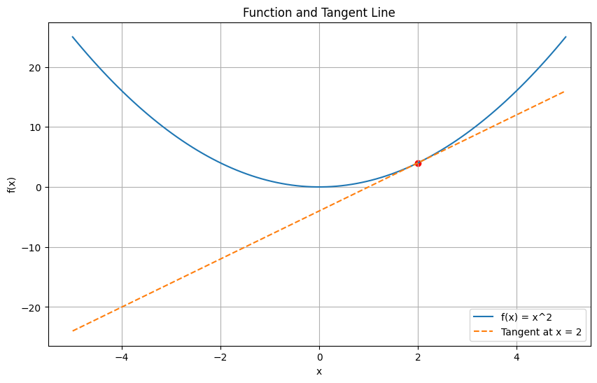
# Step 5: Visualizing the Function and its Derivative

# Visualize the function and its slope (derivative) at $x = 2$:

# Define the function and derivative as lambdas
func_lambda = sp.lambdify(x, function, 'numpy')
deriv_lambda = sp.lambdify(x, derivative, 'numpy')

# Generate x values
x_vals = np.linspace(-5, 5, 100)
y_vals = func_lambda(x_vals)
tangent_line = deriv_lambda(value_at_x) * (x_vals - value_at_x) + func_lambda(value_at_x)

# Plotting
plt.figure(figsize=(10, 6))
plt.plot(x_vals, y_vals, label='f(x) = x^2')
plt.plot(x_vals, tangent_line, label='Tangent at x = 2', linestyle='dashed')
plt.scatter(value_at_x, func_lambda(value_at_x), color='red') # point of tangency
plt.title('Function and Tangent Line')
plt.xlabel('x')
plt.ylabel('f(x)')
plt.legend()
plt.grid(True)
plt.show()
Understanding the Formula#
The derivative formula encapsulates the slope of the tangent line at any point on a function’s curve. It’s a precise measurement of the function’s rate of change at that very point, distinguishing it from an average rate of change over an interval.
Best Practices and Implementation#
Continuity Check: Ensure the function’s continuity around the point of interest.
Symbolic Computation: Use libraries like sympy for symbolic computation.
Graphical Validation: Plot your results to visualize and confirm the function and its derivative.
Conclusion#
Derivatives are fundamental in understanding and predicting changes across various domains. Their role in machine learning and AI is pivotal in optimizing models, understanding feature significance, and ensuring robust and interpretable models. Today’s lesson has imparted a thorough understanding of derivatives, their implementation, and visualization, marking a significant stride in your journey through calculus, machine learning, and AI.
Further Resources#
https://openstax.org/books/calculus-volume-1/pages/3-1-defining-the-derivative
https://towardsai.net/p/machine-learning/mastering-derivatives-for-machine-learning