
Day 17: In-Depth EDA and Central Tendency in Python#
In this lesson, we will delve into the mathematical underpinnings of central tendency, explore their practical implementation in Python, and discuss best practices for data visualization. We will also guide you on how to interpret these visualizations effectively.
Objectives:#
Understand Central Tendency: Deepen understanding of the mathematical concepts of mean, median, and mode.
Implement in Python: Learn to calculate these measures and visualize the results using Python.
Interpret Visualizations: Gain skills in reading and interpreting data visualizations.
Best Practices: Learn the do’s and don’ts of data visualization and how to apply best practices.
Prerequisites#
Intermediate Python, Pandas, NumPy, Seaborn, and Scikit-Learn skills.
Basic understanding of statistical concepts and linear algebra.
Dataset: 100daysofml/100daysofml.github.io
# Import necessary libraries
import pandas as pd
import matplotlib.pyplot as plt
import seaborn as sns
from scipy import stats
# Load the dataset
wine_data = pd.read_csv('wine_quality.csv')
1. Deep Dive into Central Tendency#
Central tendency measures give us an understanding of the typical or central value in our dataset. They are foundational in statistical analysis and EDA.
1.1 Mean (Arithmetic Average)#
Formula: \((\bar x = \frac{1}{n} \sum_{i=i}^{n} x_{i} )\)
Interpretation: Represents the average value. It considers all data points but can be heavily influenced by outliers.
Python Implementation:
mean_value = wine_data['feature_name'].mean()
1.2 Median (Middle Value)#
Formula: Middle value in a sorted list of numbers. If the number of observations is even, it’s the average of the two middle numbers.
Interpretation: Represents the middle value and is not affected by outliers or skewed data.
Python Implementation:
median_value = wine_data['feature_name'].median()
1.3 Mode (Most Frequent Value)#
Formula: The value that appears most frequently in a data set.
Interpretation: Represents the most common value. It’s the only measure of central tendency that can be used with categorical data.
Python Implementation:
mode_value = wine_data['feature_name'].mode()[0]
2. Visualization Techniques and Best Practices#
Histograms and Boxplots:#
Histograms:
Best Practices: Choose an appropriate number of bins; too few bins will oversimplify reality, too many will complicate the story.
Interpretation: Look for symmetry, skewness, and the presence of outliers.
Python Code:
wine_data['feature_name'].hist(bins=10)
plt.title('Histogram of Feature')
plt.xlabel('Feature')
plt.ylabel('Frequency')
plt.show()
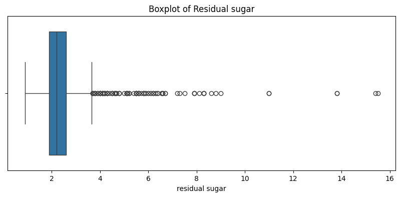
Boxplots:
Best Practices: Understand that boxplots summarize the distribution of a dataset. The box represents the interquartile range (IQR) and the line inside the box is the median. Whiskers represent the range of the data and dots outside the whiskers are considered outliers.
Interpretation: Look for the spread of the data, central value, and potential outliers.
Python Code:
sns.boxplot(x='feature_name', data=wine_data)
plt.title('Boxplot of Feature')
plt.show()
Violin Plots and Pair Plots:#
Violin Plots: Provide more information than boxplots by also showing the probability density of the data at different values.
Interpretation: Similar to boxplots but with an added layer of nuance due to the inclusion of data density.
Python Code:
sns.violinplot(x='feature_name', data=wine_data)
plt.title('Violin Plot of Feature')
plt.show()
Pair Plots: Show pairwise relationships in the dataset.
Interpretation: Look for correlations, trends, and potential clusters.
Python Code:
sns.pairplot(wine_data)
plt.title('Pairwise Relationships')
plt.show()
3. Hands-on Activities#
Activity: Comparative Analysis of Central Tendency Measures#
Objective: Compare the mean, median, and mode of key features in the Wine Quality Dataset.
Python Code:
features = ['alcohol', 'pH', 'residual sugar']
    for feature in features:
        mean_value = wine_data[feature].mean()
        median_value = wine_data[feature].median()
        mode_value = wine_data[feature].mode()[0]
        print(f"{feature} - Mean: {mean_value}, Median: {median_value}, Mode: {mode_value}")
Discussion: Evaluate how these measures differ for each feature and hypothesize why that might be the case.
4. Homework Assignment#
Task: Students are required to perform a comparative analysis of central tendency and dispersion for three variables from the Wine Quality Dataset. They should:
Calculate mean, median, mode, variance, and standard deviation.
Create histograms and boxplots for each variable.
Write a brief report, comparing these measures and discussing their implications for wine quality.
Best Practices for Reporting:#
Clarity: Make sure your visualizations are clear and your narrative is easy to follow.
Context: Provide context for your findings. Numbers and plots are meaningless without interpretation.
Accuracy: Ensure your calculations are correct and your interpretations are based on the data.
Homework - Solution#
# Import necessary libraries
import pandas as pd
import matplotlib.pyplot as plt
import seaborn as sns
from scipy import stats

# Load the dataset
wine_data = pd.read_csv('wine_quality.csv')
# List of features to analyze
features = ['alcohol', 'pH', 'residual sugar']
# Initialize a dictionary to store the results
analysis_results = {}
# Loop through each feature and calculate statistics
for feature in features:
    # Calculating Descriptive Statistics
    mean_value = wine_data[feature].mean()
    median_value = wine_data[feature].median()
    mode_value = wine_data[feature].mode()[0]
    variance_value = wine_data[feature].var()
    std_dev_value = wine_data[feature].std()

    # Storing the results
    analysis_results[feature] = {
        'mean': mean_value,
        'median': median_value,
        'mode': mode_value,
        'variance': variance_value,
        'std_dev': std_dev_value
    }
# Plotting Histogram
plt.figure(figsize=(10, 4))
wine_data[feature].hist(bins=15)
plt.title(f'Histogram of {feature.capitalize()}')
plt.xlabel(feature.capitalize())
plt.ylabel('Frequency')
plt.grid(False)
plt.show()
# Plotting Boxplot
plt.figure(figsize=(10, 4))
sns.boxplot(x=feature, data=wine_data)
plt.title(f'Boxplot of {feature.capitalize()}')
plt.show()
# Displaying the analysis results
for feature, stats in analysis_results.items():
    print(f"\nStats for {feature.capitalize()}:")
    for stat_name, stat_value in stats.items():
        print(f"{stat_name.capitalize()}: {stat_value}")
Stats for Alcohol:
Mean: 10.442111402741325
Median: 10.2
Mode: 9.5
Variance: 1.1711473380358497
Std_dev: 1.0821956098764445
Stats for Ph:
Mean: 3.3110148731408575
Median: 3.31
Mode: 3.3
Variance: 0.02454362762448039
Std_dev: 0.15666405977275194
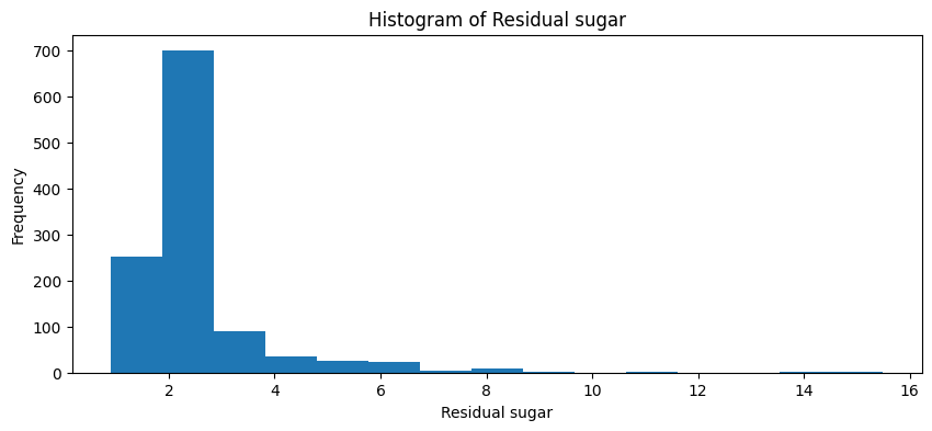
Stats for Residual sugar:
Mean: 2.5321522309711284
Median: 2.2
Mode: 2.0
Variance: 1.8385121764551762
Std_dev: 1.3559174666826799
Report Template#
Comparative Analysis of Central Tendency and Dispersion for Wine Quality Variables#
Introduction:#
This report presents a comparative analysis of the central tendency (mean, median, mode) and dispersion (variance, standard deviation) for three key variables (alcohol, pH, residual sugar) from the Wine Quality Dataset.
Findings:#
Alcohol:
Central Tendency:
Mean: [mean_value]
Median: [median_value]
Mode: [mode_value]
Dispersion:
Variance: [variance_value]
Standard Deviation: [std_dev_value]
Histogram Analysis: [Provide analysis based on histogram]
Boxplot Analysis: [Provide analysis based on boxplot]
pH:
Central Tendency:
Mean: [mean_value]
Median: [median_value]
Mode: [mode_value]
Dispersion:
Variance: [variance_value]
Standard Deviation: [std_dev_value]
Histogram Analysis: [Provide analysis based on histogram]
Boxplot Analysis: [Provide analysis based on boxplot]
Residual Sugar:
Central Tendency:
Mean: [mean_value]
Median: [median_value]
Mode: [mode_value]
Dispersion:
Variance: [variance_value]
Standard Deviation: [std_dev_value]
Histogram Analysis: [Provide analysis based on histogram]
Boxplot Analysis: [Provide analysis based on boxplot]
Discussion:#
Discuss the implications of the central tendency and dispersion measures on the quality of wine. How do these variables influence the wine quality, and what could be the potential reasons for the observed patterns?
Conclusion:#
Summarize the key insights obtained from the analysis and suggest any potential actions or further analyses that could be beneficial for wine producers or marketers.
**Additional Resources (In Depth EDA & Central Tendency)#
https://econometricstutors.com/exploratory-data-analysis-central-tendency/
https://www.geeksforgeeks.org/exploratory-data-analysis-eda-types-and-tools/